How to Collect Unemployment Data for all the US States from FRED
FRB (Federal Reserve Bank) collects tons of economic data (765,000!) such as Unemployment Rate, GDP, Treasury Rate, etc. and amazingly, it publishes the data on their website called FRED (Federal Reserve Bank Economic Data) for public access.
And, if you are an R user, there is good news!
There is an R package called ‘tidyquant’, which makes it super easy to get such data directly from the FRED!🔥
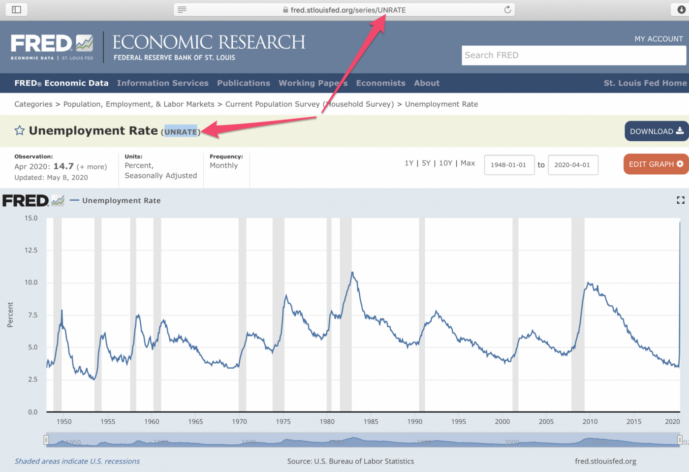
For example, if you want to get the US national level unemployment rate all you need is the following code.
library(tidyquant)

tq_get("UNRATE", get = "economic.data", from = "1999-01-01")
I’m going to use Exploratory to demonstrate here.
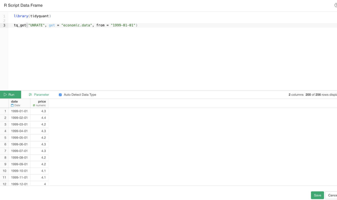
The 1st parameter inside the ‘tq_get’ function is the code for the data. In this case, that is the code for the Unemployment Rate data.
You can find the code on the unemployment rate page at FRED.
Collect Data for All US States
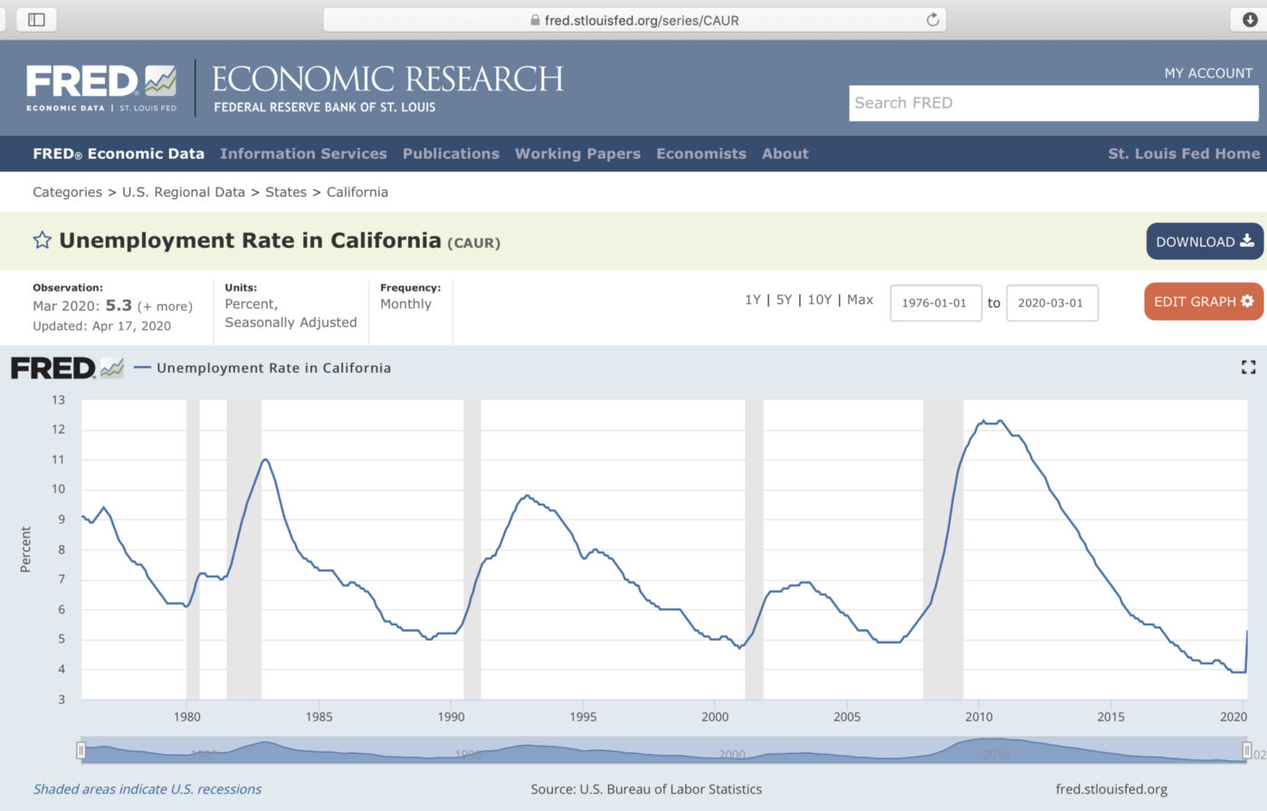
Now, there are also US State-level unemployment data. For example, this page is for the unemployment rate in California.
You can, of course, get this data by running an R command like the below.
tq_get("CAUR", get = "economic.data", from = "1999-01-01")Now, what if we want to get all the 50 states data?
This requires a bit of coding, but it’s relatively straightforward.
First, the code for the state-level unemployment rate has the following rule.
<State_Code>URFor example, it is ‘CAUR’ for California and ‘NYUR’ for New York, etc.
So we can run the above ‘tq_get’ function 50 times, and each time we run it we can replace the code for each state.
And, instead of manually copying & pasting the code, we can automate it by creating a function.
Here is such a function called “download_all_states”.
download_all_states <- function(state_code) {
  fred_code <- str_c(state_code, "UR")

  tq_get(fred_code, get = "economic.data",
         from = "1999-01-01") %>%
  mutate(state = state_code)
}
This ‘download_all_states’ function does the following 4things.
- takes an argument called ‘state_code’.
- use the value of the argument ‘state_code’ and concatenate with “UR” to construct the code for each state, and put the value into ‘fred_code’ variable.
- pass the fred_code variable to the ‘tq_get’ function as the code argument.
- add ‘mutate’ command to create a new column to store the state code value.
Once we have this function then we can create an iterative process for calling this function 50 times.
And in R, there is this cool package called ‘purrr’, which provides a function called ‘map_dfr’, which calls a given function as many as a number of values in a given list.
Here is how you can use it.
map_dfr(state_list, download_all_states)The ‘state_list’ is supposed to be a list with all the 50 State codes.
The ‘map_dfr’ function calls the ‘download_all_states’ function 50 times (50 States) and passes the value of the ‘state_list’ to the function each time.
Create a list of 50 US States
Now, how can we come up with the list of the 50 States?
It turned out that we have this list already in R!
It’s called ‘state.abb’. When you start an R session there are a few sample data and lists already loaded in the memory. And the ‘state.abb’ is one of them.
If I just type ‘state.abb’ it will return something like below.
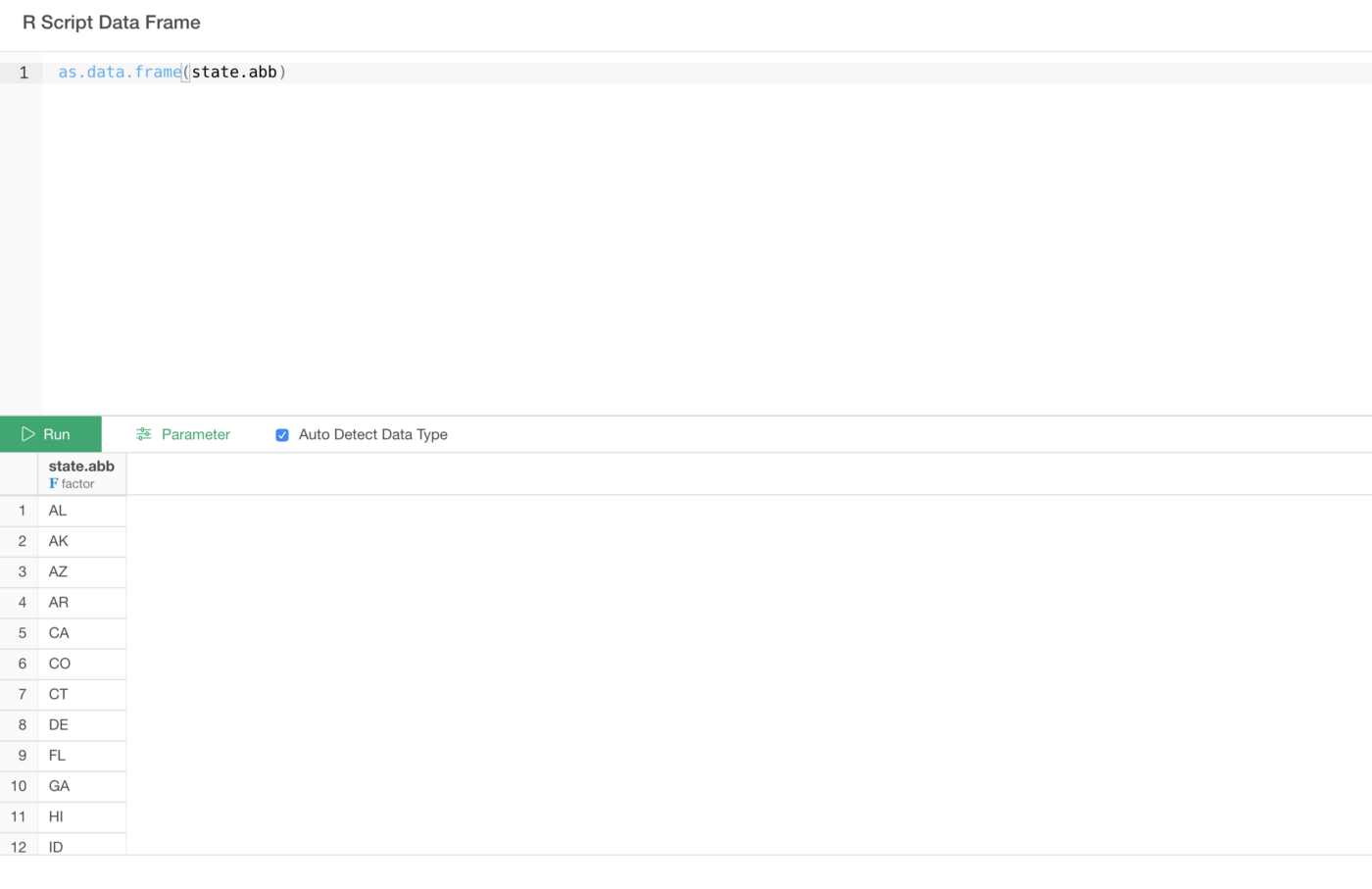
state.abb is a list (or vector) so I needed to use ‘as.data.frame’ to return the result in a data frame format inside R Script Data Source in Exploratory.
Anyway, now we can just use this ‘state.abb’ as the 1st argument of the ‘map_dfr’ function like below.
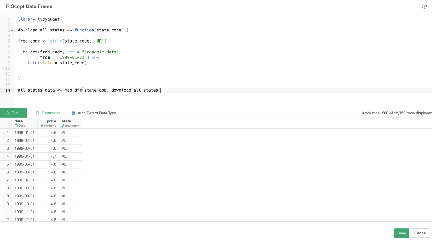
map_dfr(state.abb, download_all_states)So, the whole code would look something like below.
library(tidyquant)

download_all_states <- function(state_code) {

fred_code <- str_c(state_code, "UR")

  tq_get(fred_code, get = "economic.data",
         from = "1999-01-01") %>%
  mutate(state = state_code)
}

all_states_data <- map_dfr(state.abb, download_all_states)
Run the Script and Import the Data
And now, we can run the whole thing.
Once we click on the ‘Save’ button we have the whole data imported!
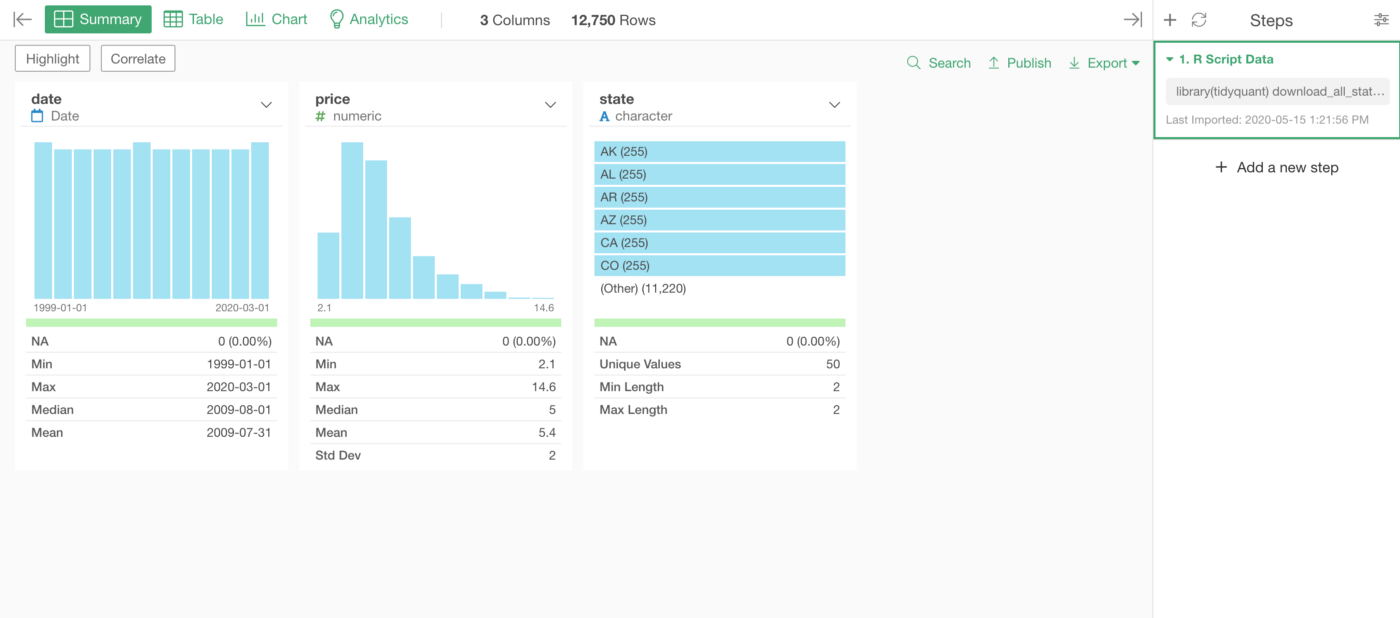
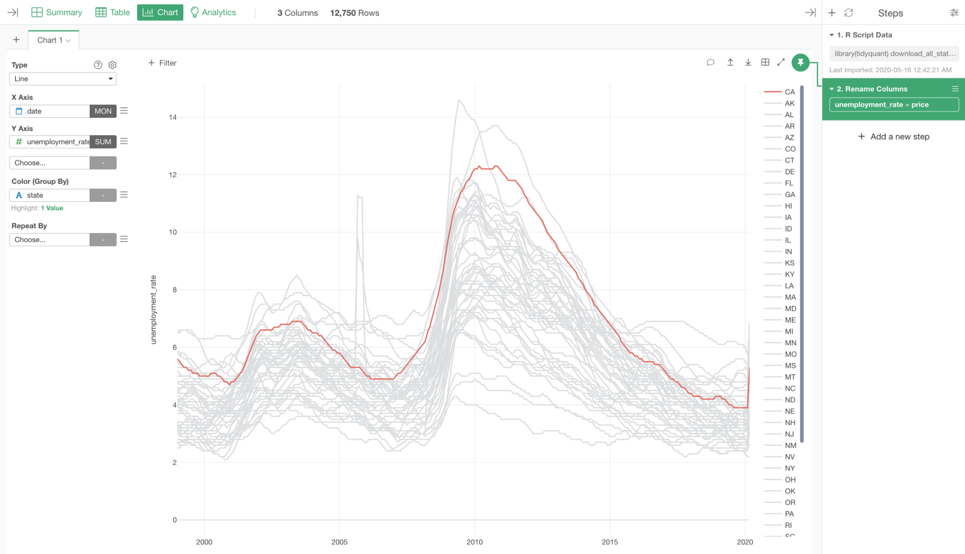
The data is from 1999-01–01 to 2020–03–01, and there are 50 states.
Rename the Column Names
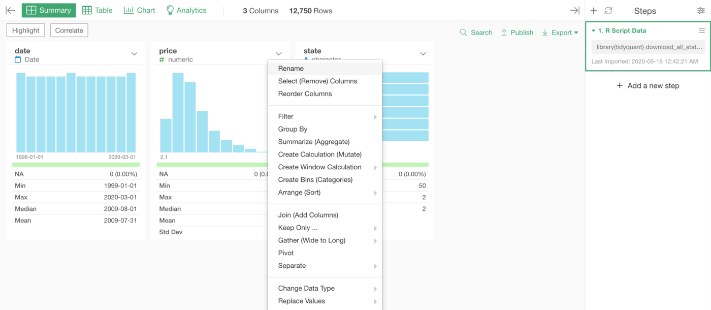
The column name for the unemployment rate is labeled as ‘price’, which we can change with the ‘Rename’ step.
Select ‘Rename’ from the column header menu.
Type something like ‘unemployment_rate’ for the price column.
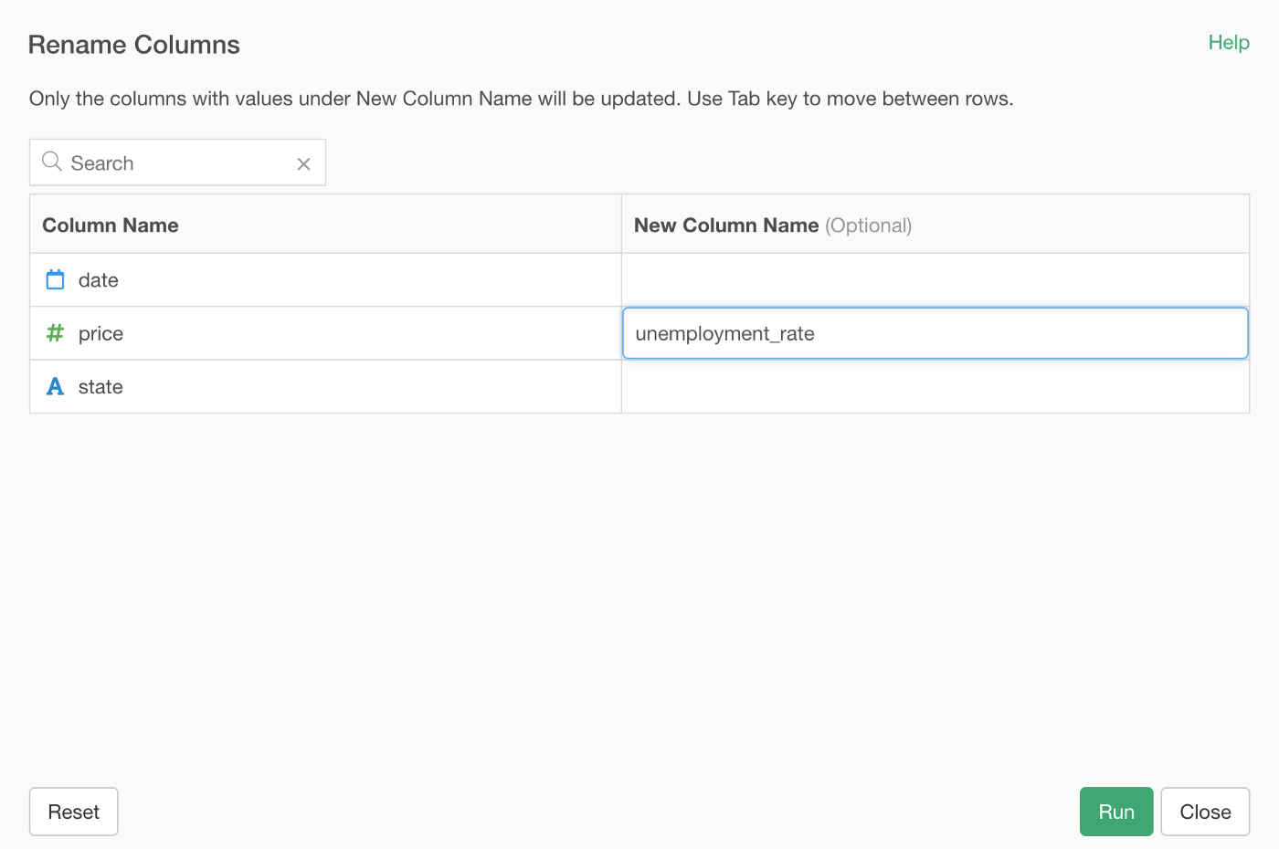
Then, you’ll get the new column name.
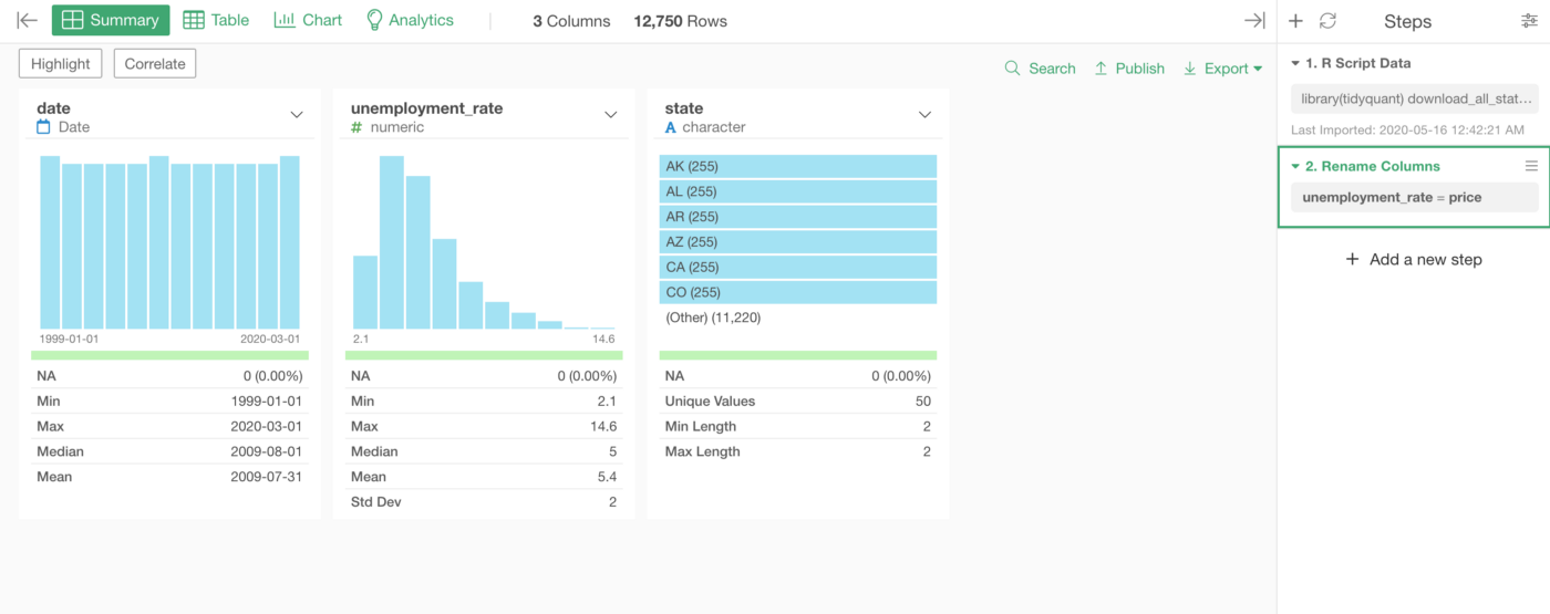
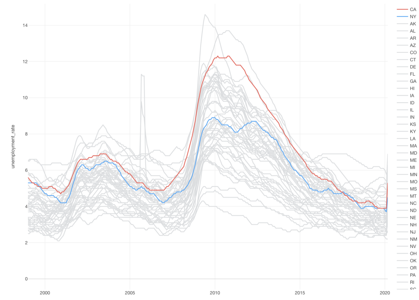
Visualize the Data
You can now visualize the data the way you like under the Chart view.