Marketing Mix Modeling with Exploratory

In this Note, I will explain how to build Marketing Mix Model with Exploratory (only with UI!), and predict future sales volume given a future marketing and pricing plan.

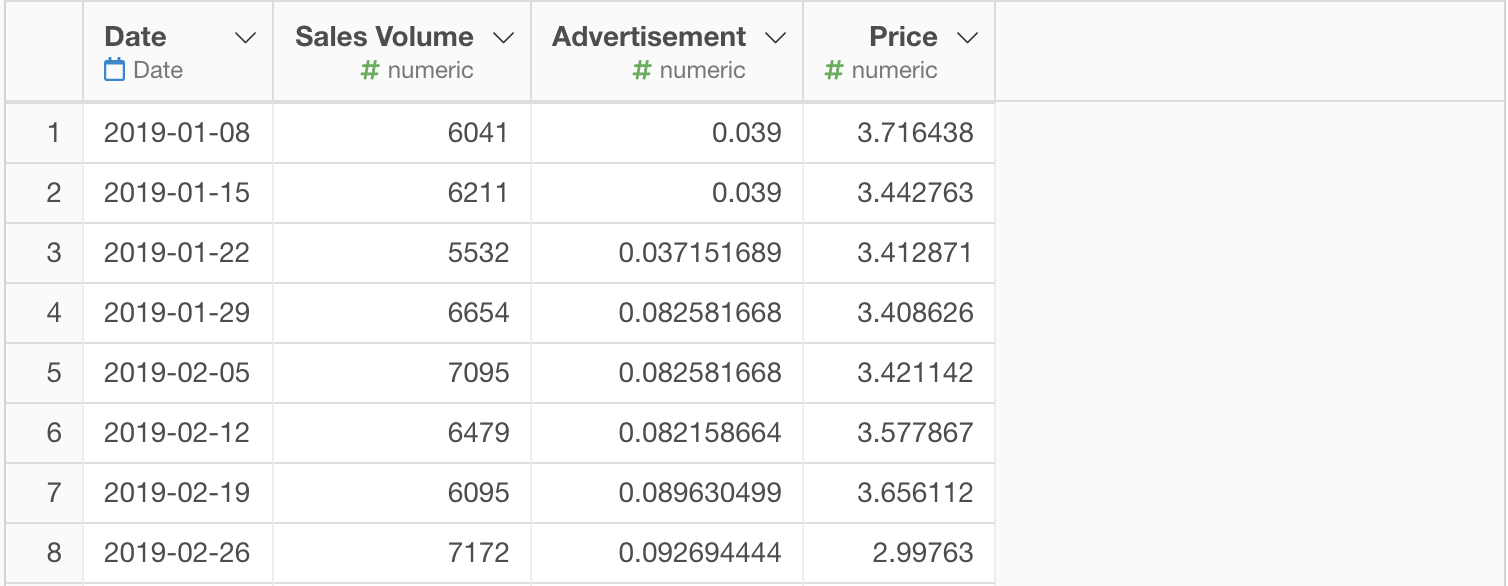
Data

Let's use a sales data of a cheese product at a super market store for our exercise. It's a weekly data of sales volume, how much advertisement was done, and the price the product was sold at.

Linear Regression

Let's start with a linear regression model to predict sales, simply from the price and advertisement of the same week.

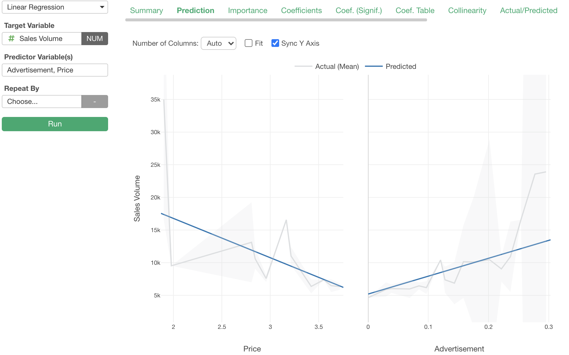
Here is the Linear Regression Analytics View predicting Sales Volume from Advertisement and Price.

We can see that Sales Volume goes down as the Price goes up, and it goes up as the Advertisement goes up, which makes common sense.

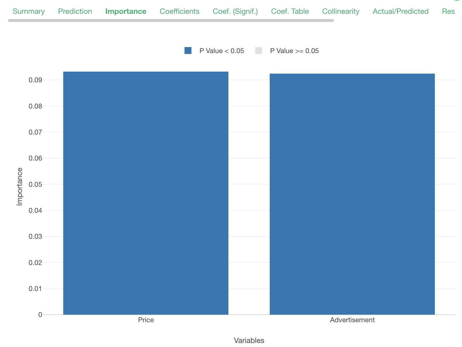
Looking at the permutation importance result on the Importance tab, it seems that the pricing and the advertisement are of same importance in terms of affecting the sales volume.

You can check the model summary info such as R squared at the Summary view. With this simplistic model, R squared is 0.656, which means that about 66% the variability of the sales volume can be explained by price and advertisement.

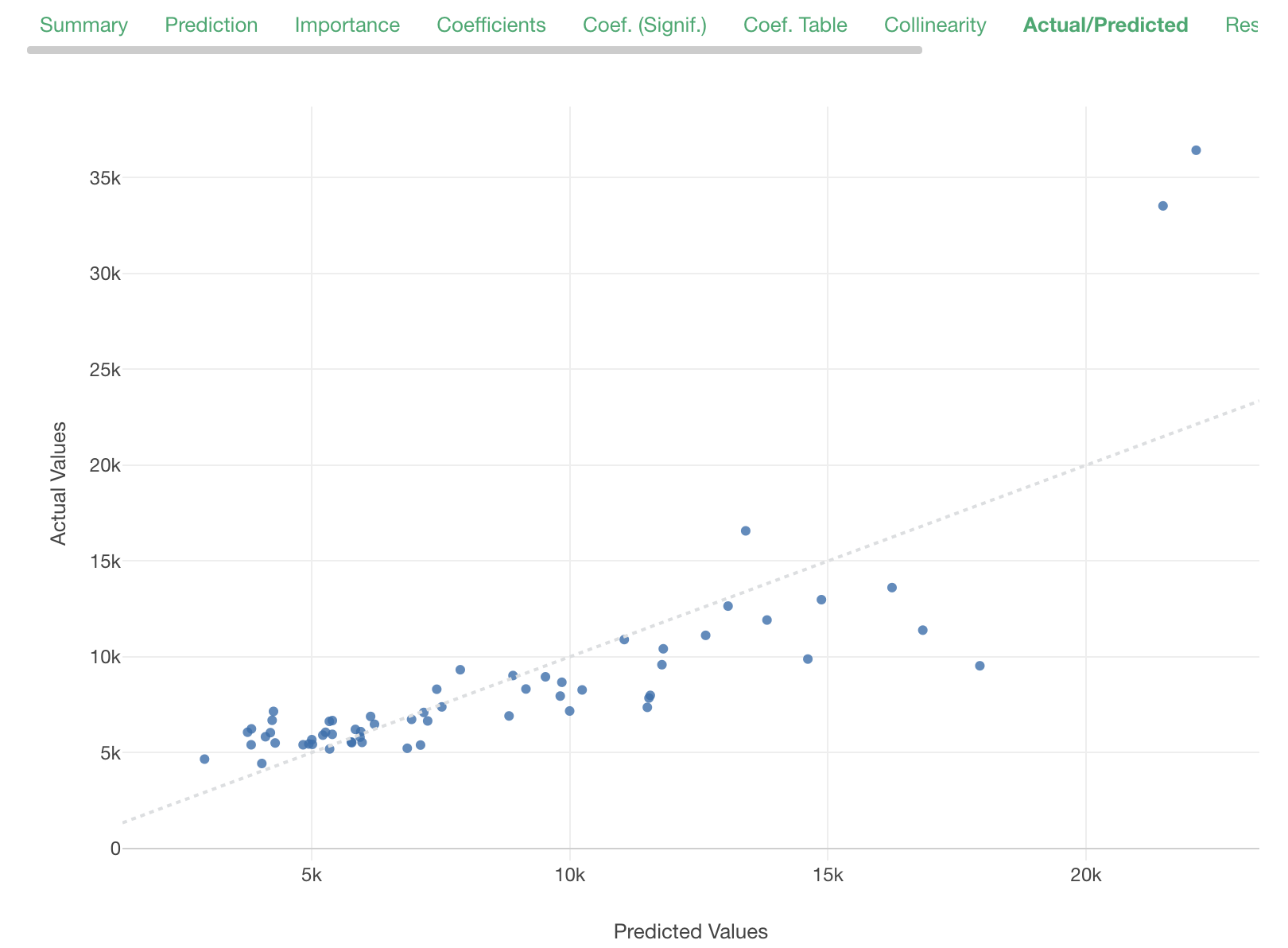
But looking at Actual/Predicted tab, it seems that the actual values are not really distributed around the predicted value. The relationship between them does not look very linear.

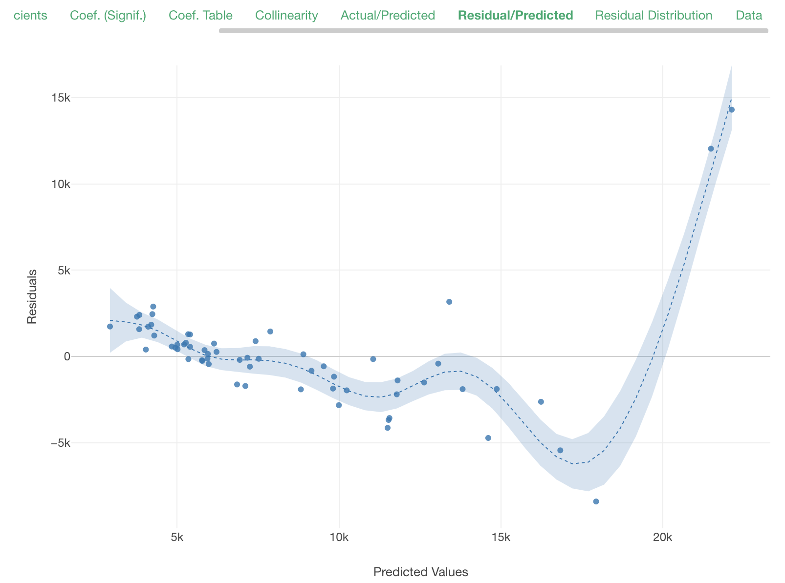
The Residual/Predicted plot reveals the same concern. The residuals are not evenly distributed above and below 0.

Using Log Scale on Sales and Price

Let's think what we can do to improve this model. It seems that price has significant impact on the sales volume with this model.

Here, by simply applying linear regression for the relationship between price and sales, we have been implicitly assuming that price and sales have additive linear relationship. But more commonly accepted model for relationship between price and sales is price elasticity being a constant, which means price and sales have multiplicative relationship.

Let's take that into account in this model. To do so, you can apply log function to both the Price and the Sales Volume.

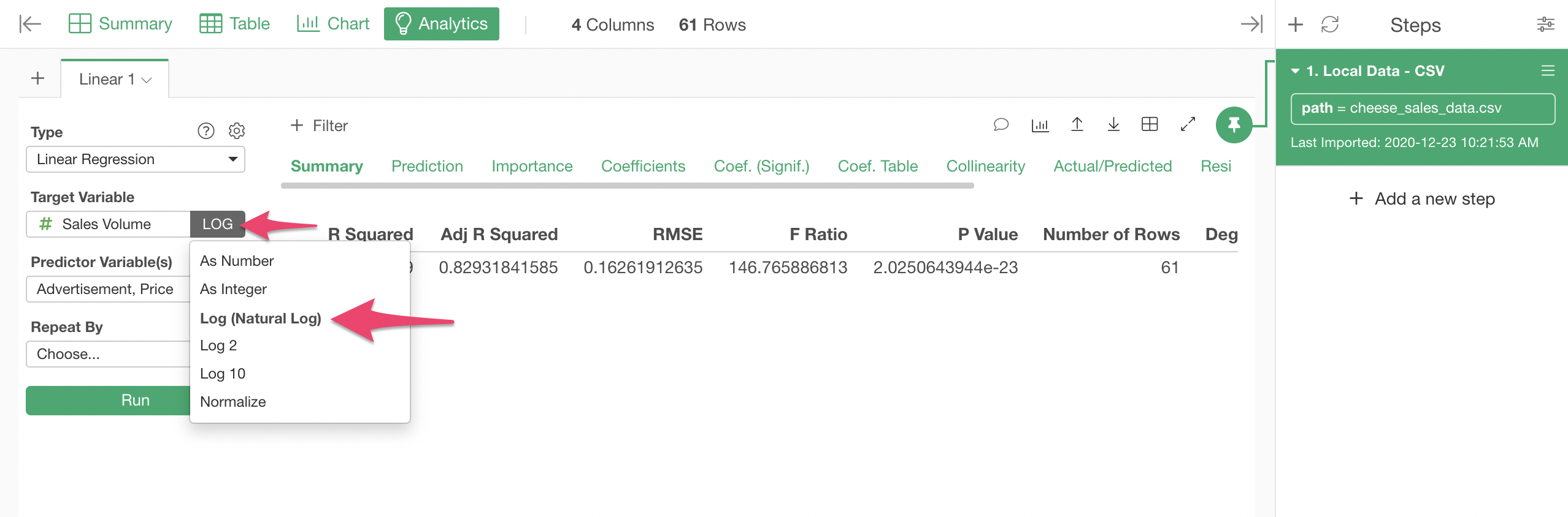
Let's apply log to the Sales Volume from the Function dropdown of the Target Variable selector.

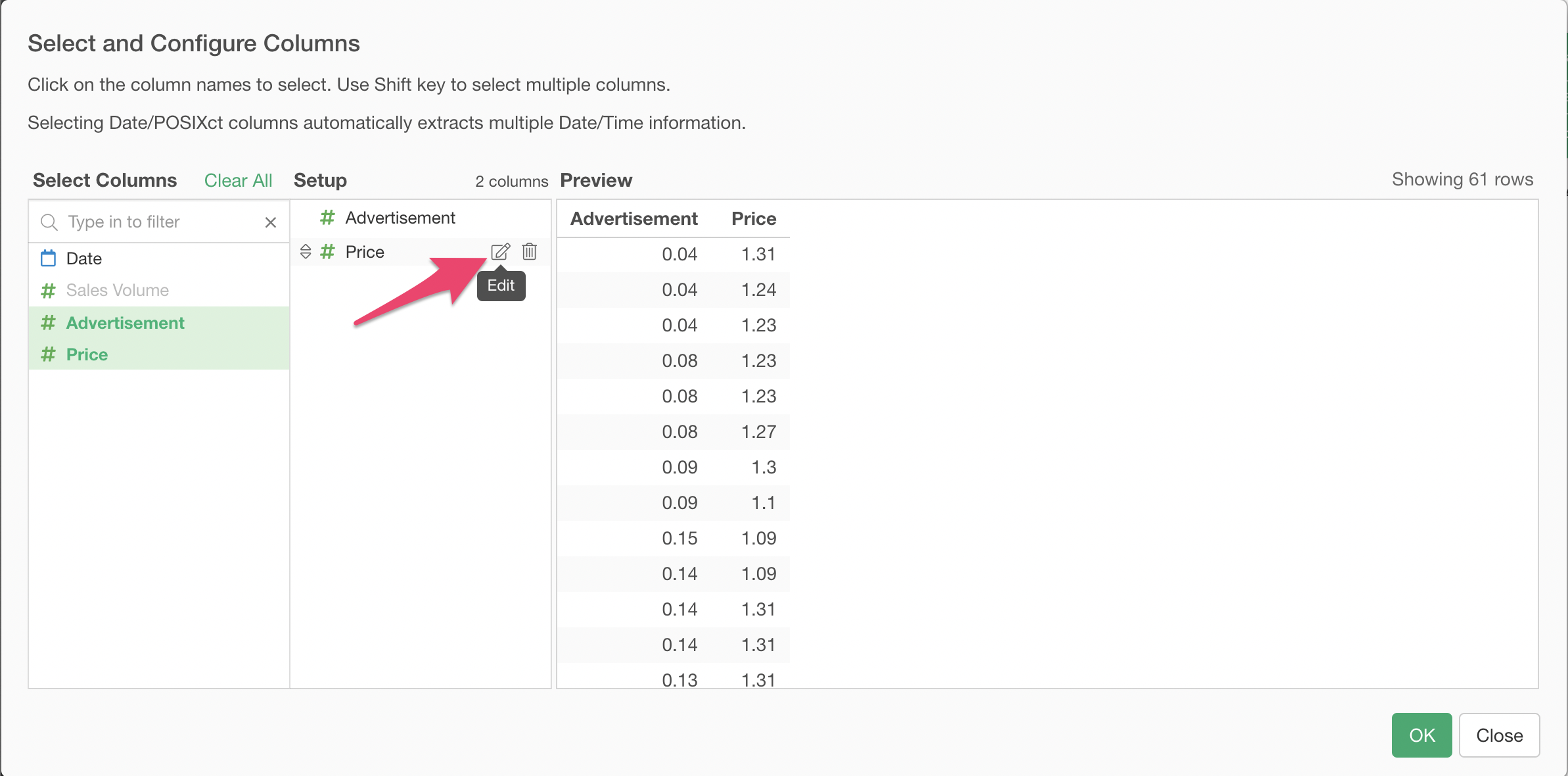
For the Price, open the Predictor Variables Selector dialog, and click the Edit icon of the Price variable.

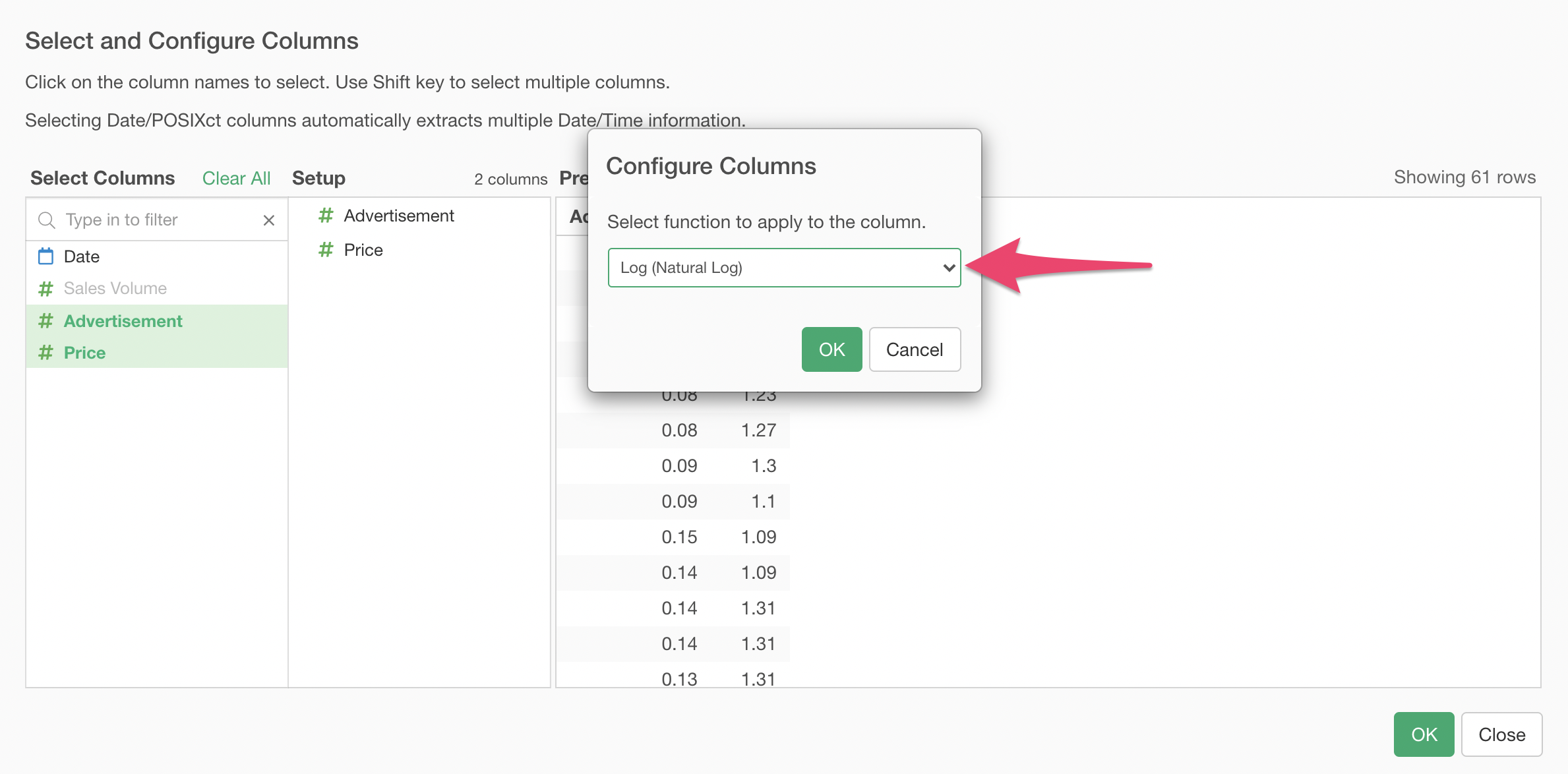
Select Log (Natural Log) function, so that it is applied to the Price before it is fed to the linear regression model.

Looking at the Actual/Predicted plot after rebuilding the model, now the distribution of data seems more in line with the perfect fit diagonal reference line.

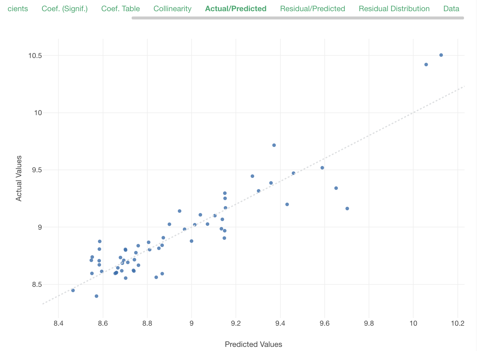
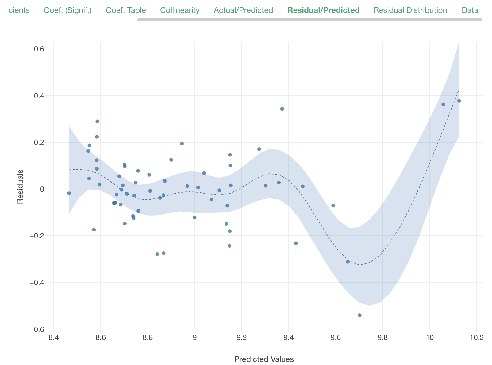
The residuals seems to be distributed more evenly between above 0 and below 0. It seems that this model represents the mechanism of price and advertisement affecting sales volume better than our previous model.

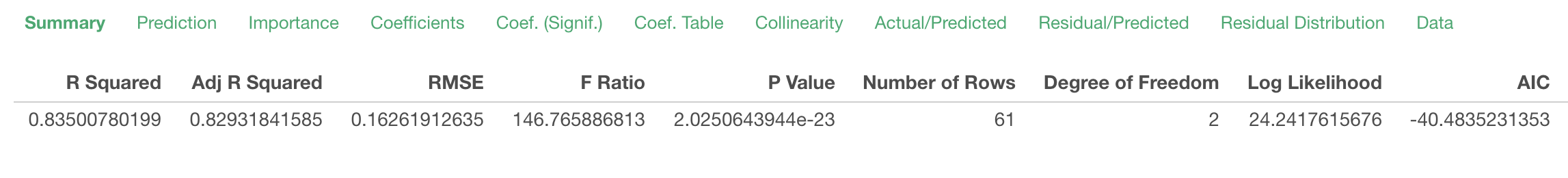
R squared is now 0.835, which is better than the previous model, though it is not apple-to-apple comparison since what we are predicting now is log of sales volume, which is different from raw sales volume.

Taking Carry Over Effect (Adstock) into Account

When we invest on advertisement effort, it is natural to expect the effect of it to last for a while, while it is remaining in people's collective memory. The advertisement done in the last week or 2 weeks ago can reasonably affect the sales of this week. This is called carry over effect of advertisement.

Our previous model did not take the carry over effect into accout at all, since we predicted the sales purely based on the same week's advertisement effort.

Let's take the carry over effect into account in our model.

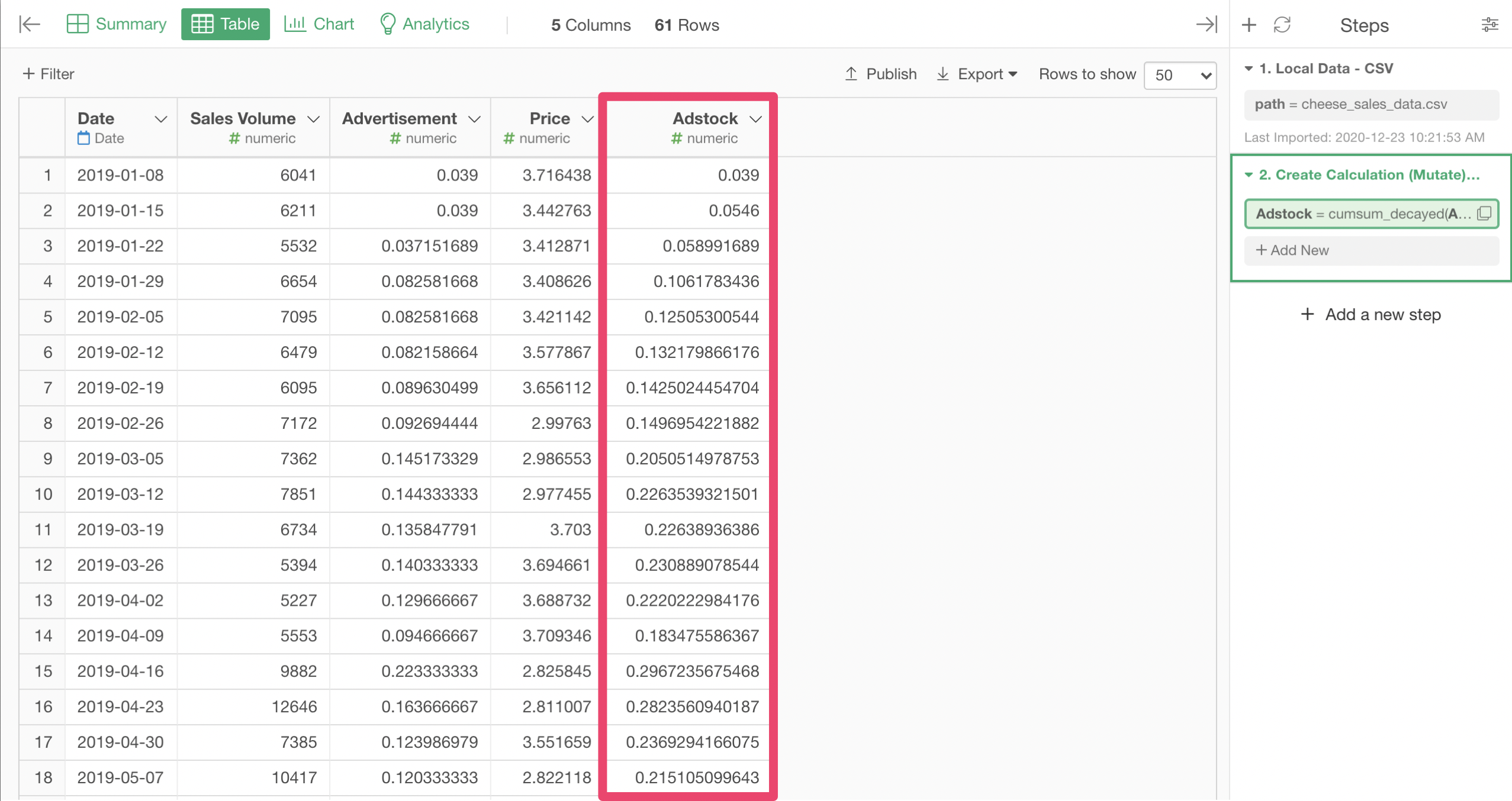
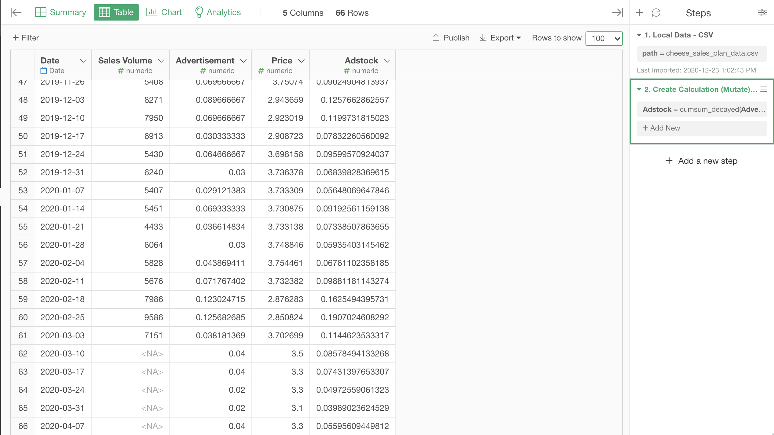
To do so, let's first calculate total effect of advertisement from the current week as well as the past weeks. This value is called "adstock".

There are many way to estimate it, but one way is assuming that the effect of advertisement at one point of time to decay at a same rate as the time goes by. For example, let's say a certain advertisement done this week had effect of 1. Next week the effect still remains, but it will decay and becomes half of it, which is 0.5. The following week, it decays further and becomes half of it again, which is 0.25, and this process goes on. And the adstock can be estimated as the sum of such decayed advertisement effect, plus the effect from advertisement of the same time.

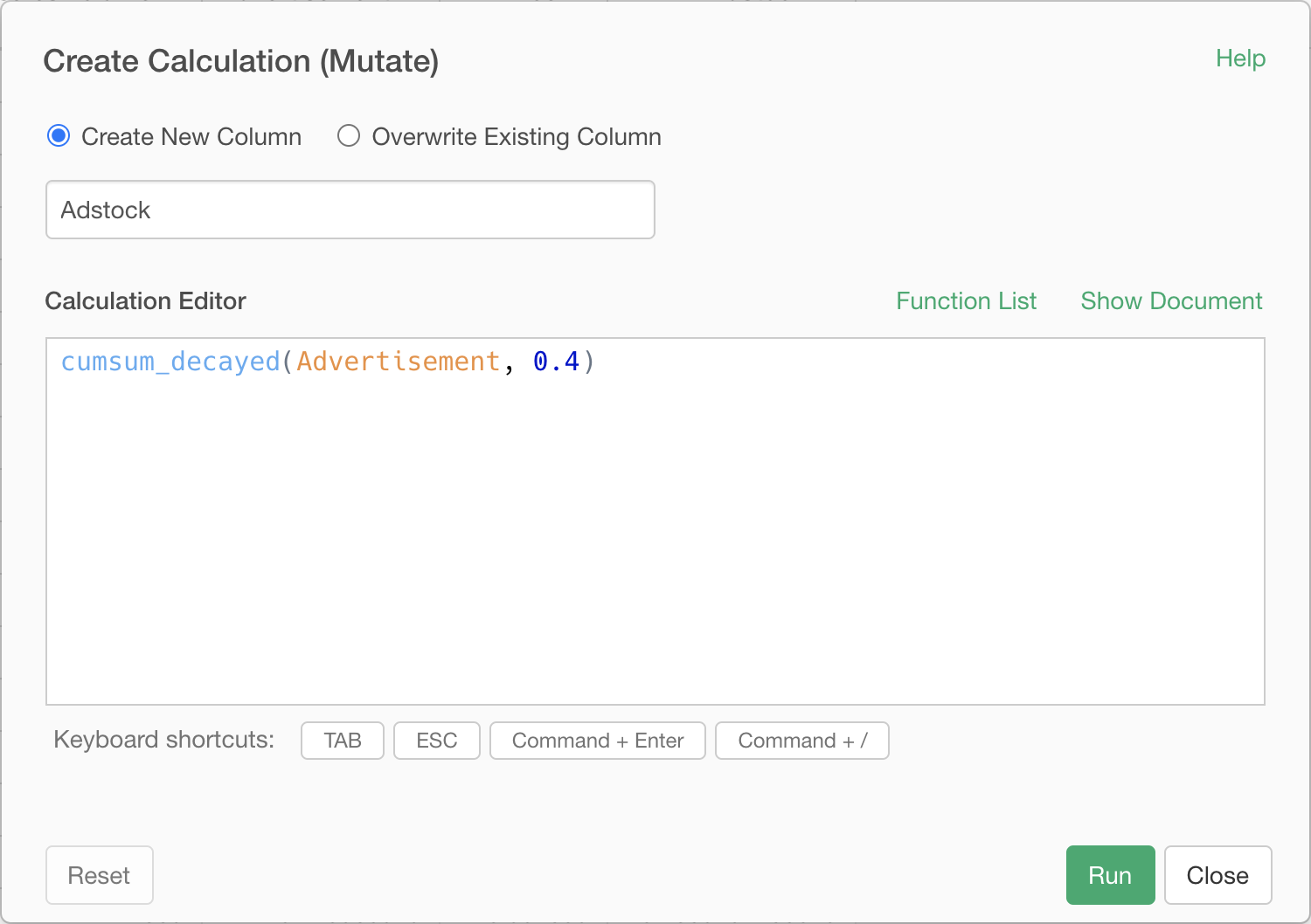
On Exploratory, this can be calculated with cumsum_decayed function. Assuming that 0.4 times the current advertisement effect is carried over to the next week, the adstock is calculated with the following expression.

cumsum_decayed(Advertisement, 0.4)

If the version of Exploratory you are using do not have cumsum_decayed function yet, you can define it by creating a Script and pasting the following in it and running it.

cumsum_decayed <- function(x, decay) {
  purrr:::accumulate(x, function(x,y){x*decay+y})
}

Let's create a Calculation (mutate) step that calculates it.

Adstock column is added.

Go back to the Analytics View, and drag/drop the Pin icon to the new step with Adstock to associate it to the new step, and select Adstock as the predictor instead of the raw Advertisement.

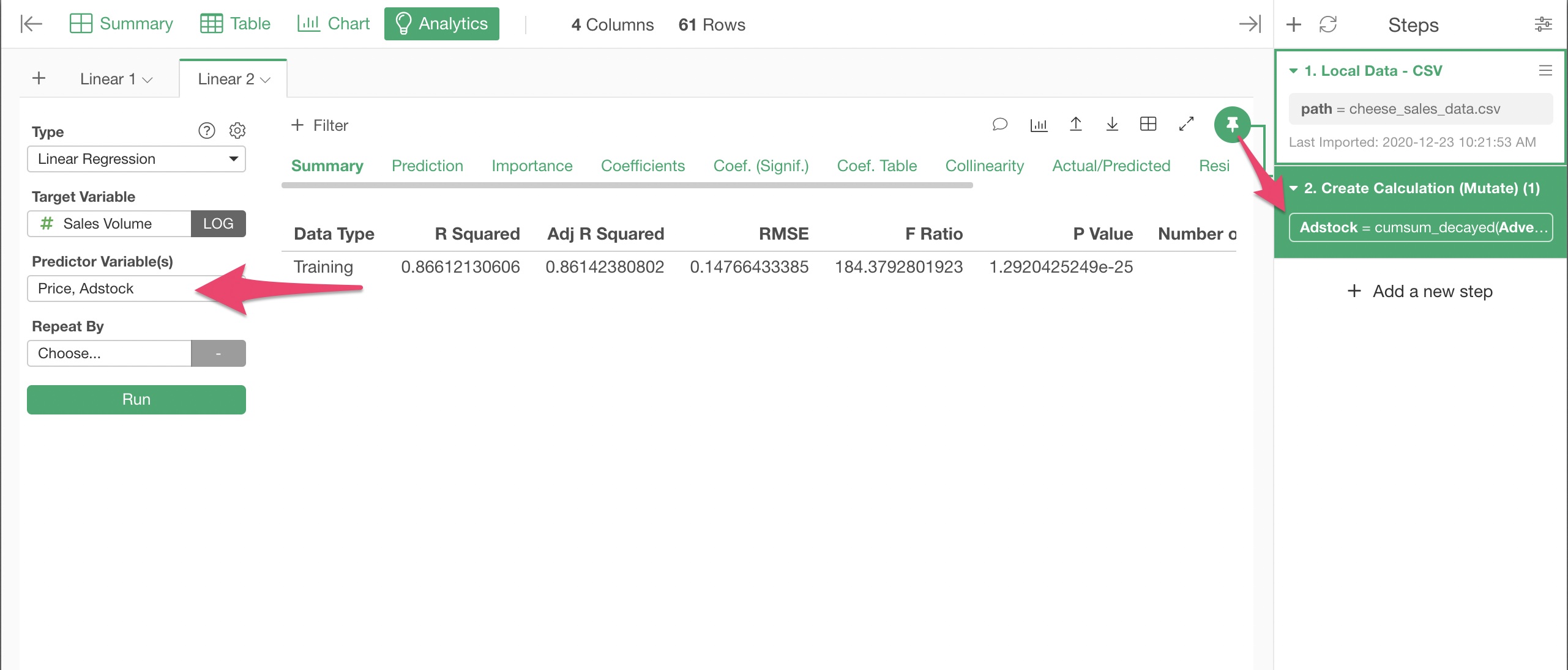
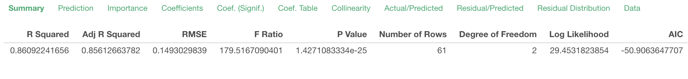
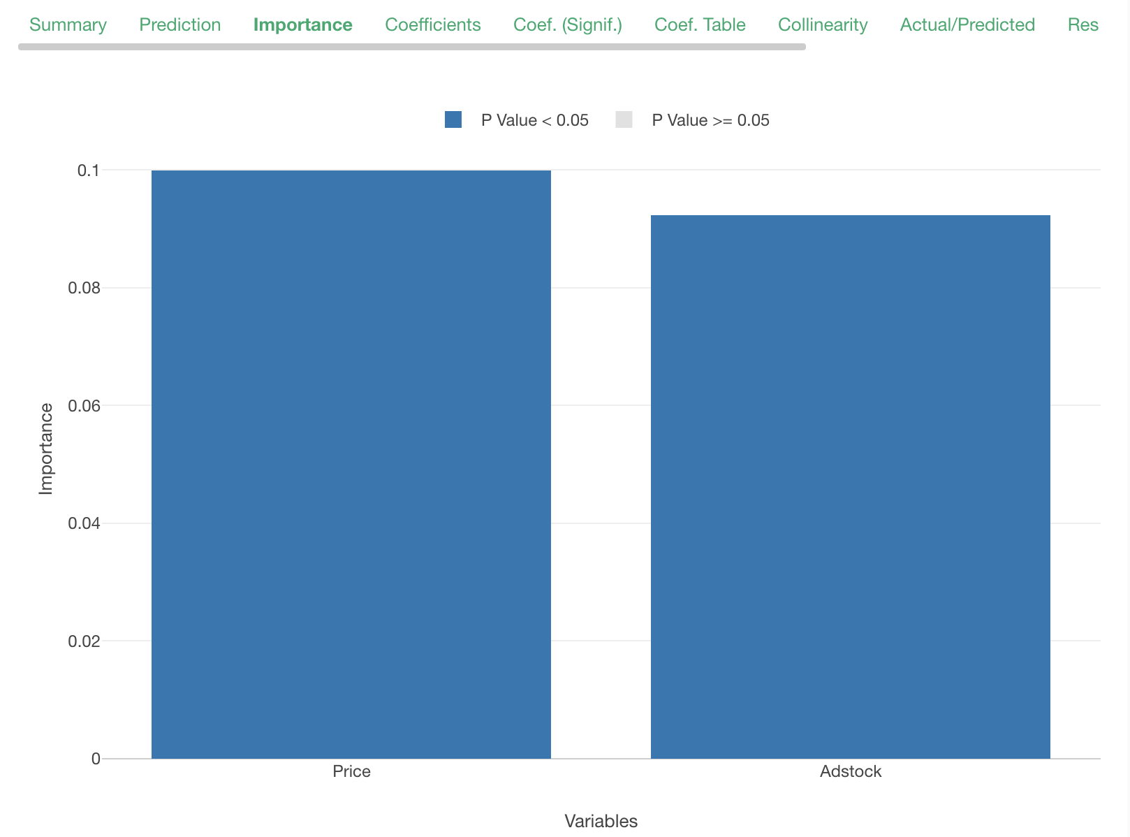
Looking at the Summary tab, we can see that the R Squared improved a little, from 83.5% to 86%.

The Actual/Predicted plot seems to be inline with the diagonal perfect fit line, just like the previous model.

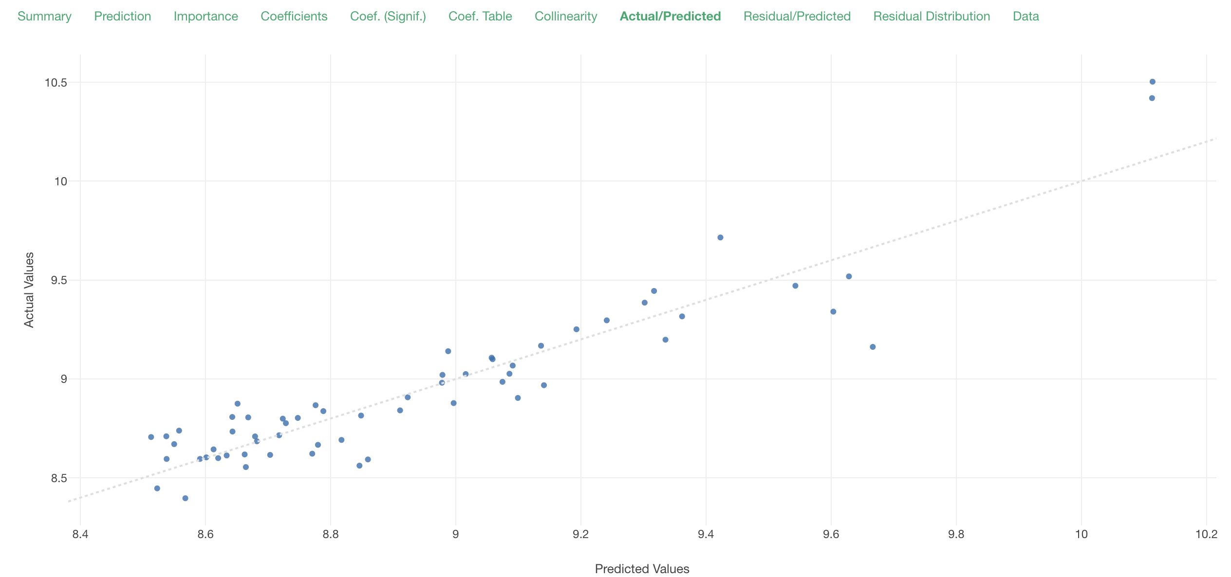
The Residual/Predicted plot looks as good as the previous model too.

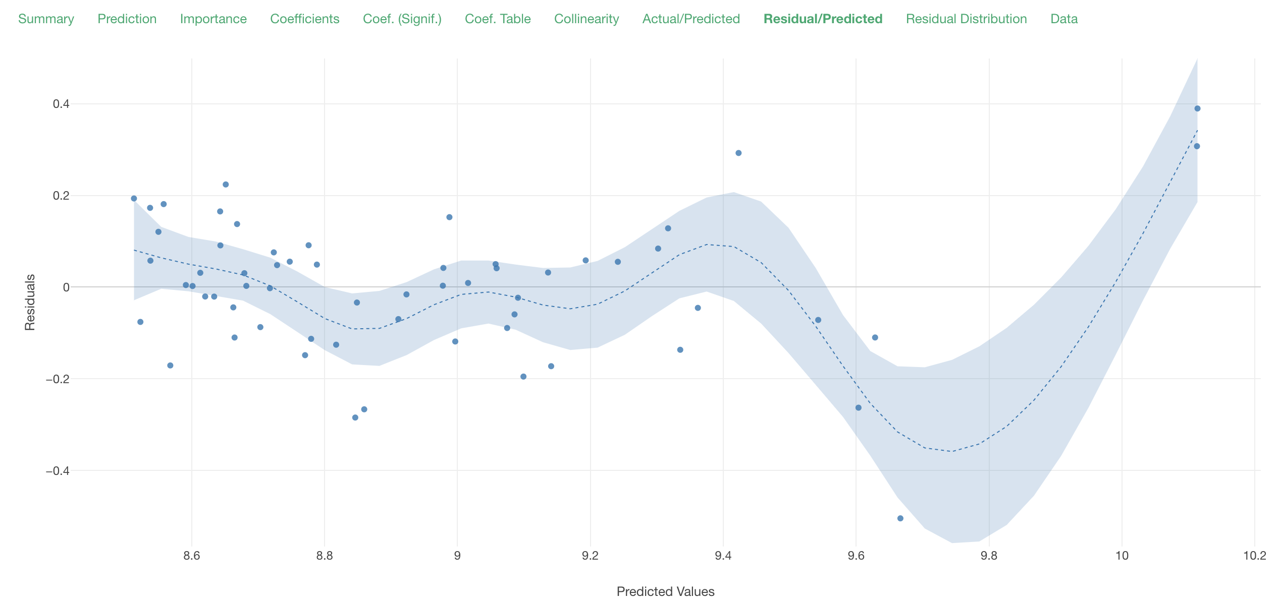
With this model, the price seems to be considered a little more important than advertisement.

Testing the Model

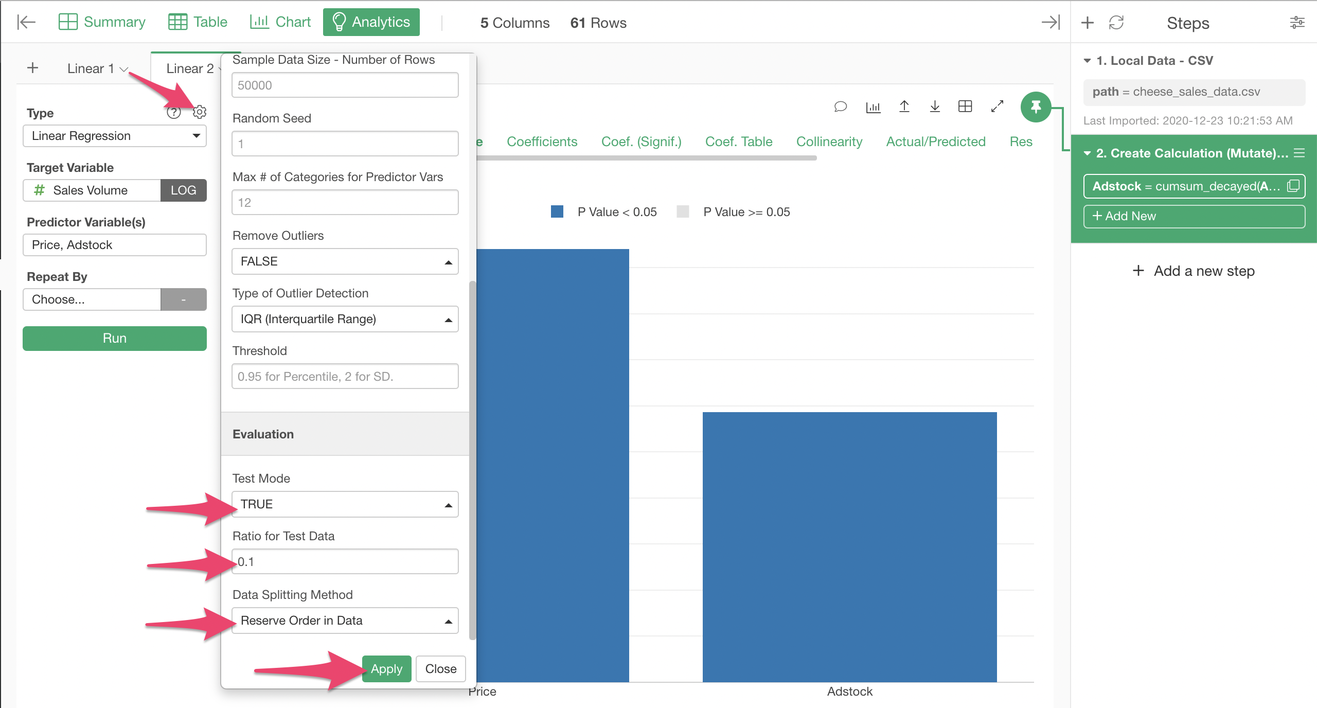
Let's test the prediction capability of this model, by using the last portion of the data as the test data.

To do this in Exploraoty, enable Test Mode from the Analytics Properties dialog.

Let's use last 10% of the period that is covered with this data for the test purpose by specifying 0.1 to the Ratio for Test Data.

By specifying "Reserve Order in Data" for Data Splitting Method, we can make sure that the last part of the data is used for the test, as opposed to random rows in the data getting used for the test.

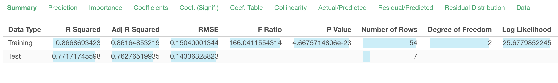
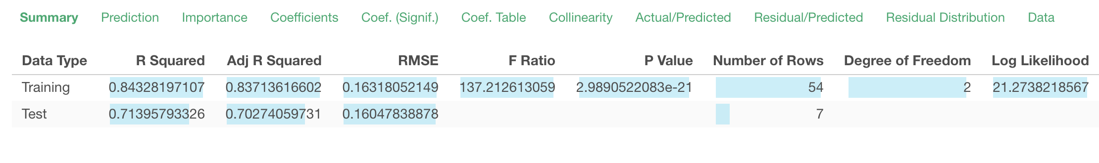
The Summary tab shows metrics of the model with the training data as well as the test data. R squared with the test data is a little lower than the one with the training data, which is expected.

Let's export the data with the prediction result as a new data frame to visualize it with a line chart as a time series data.

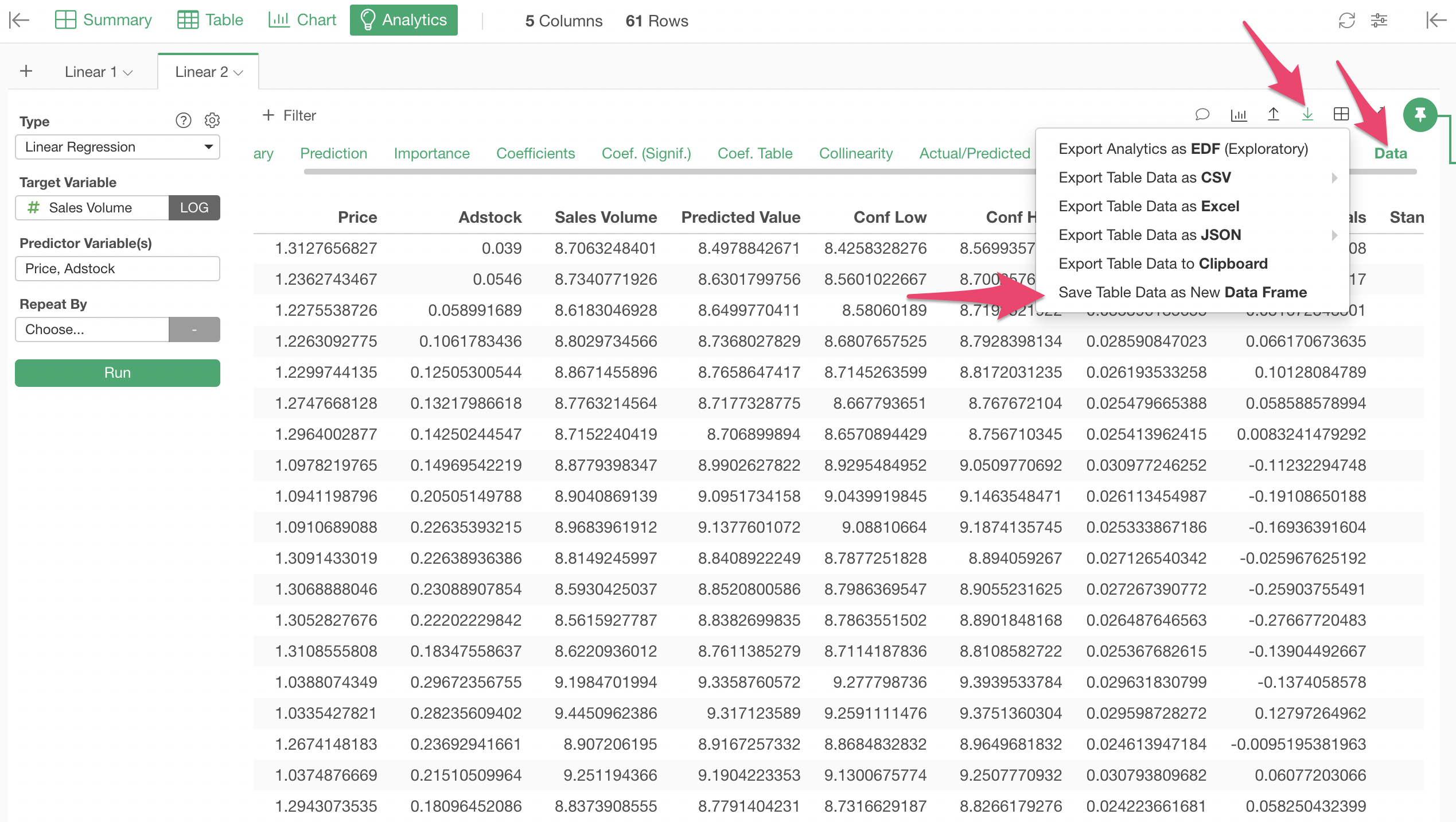
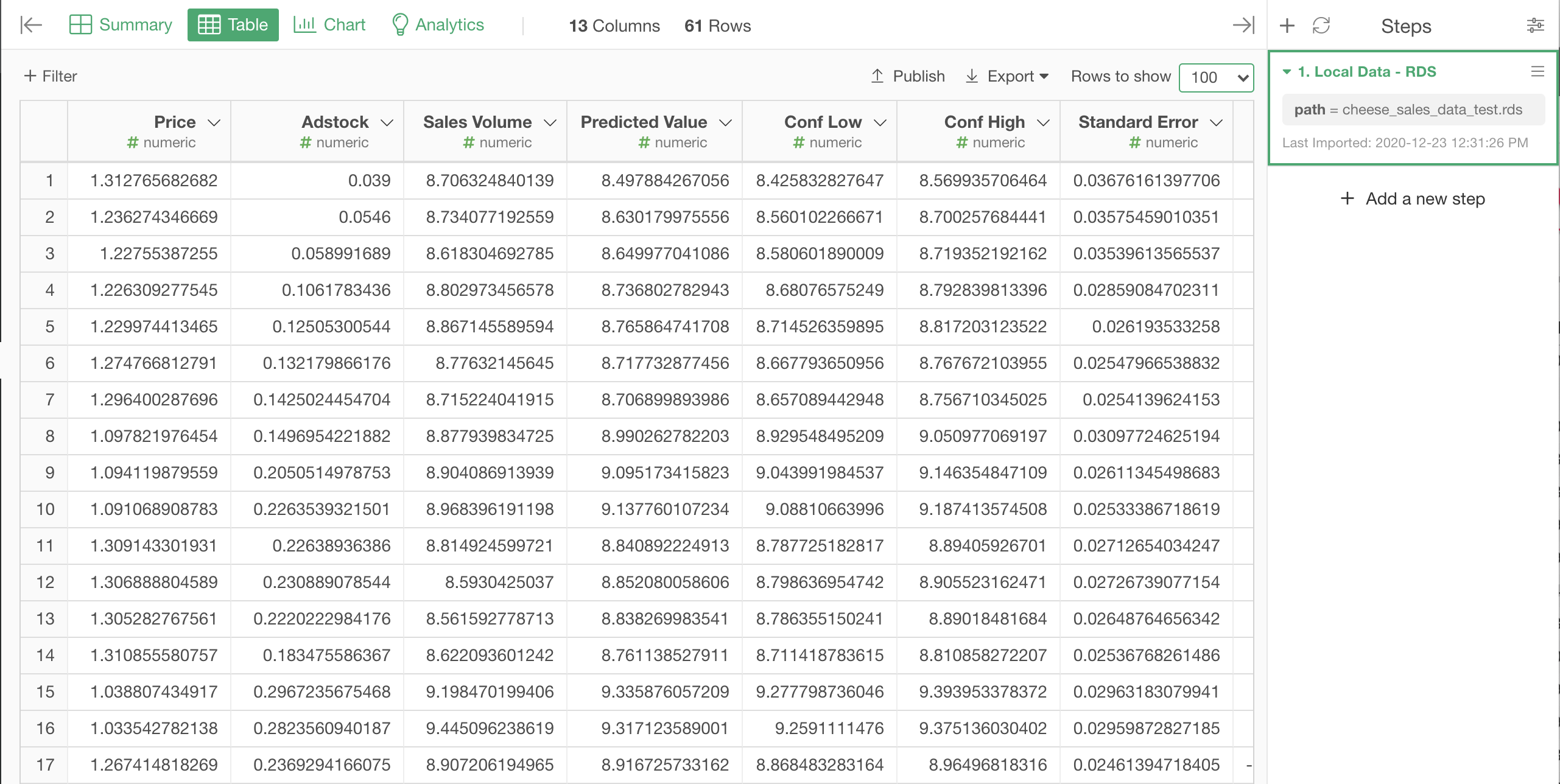
A new Data Frame is created. It holds the new columns for the prediction result, as well as the columns from the original data, although the Date column is missing here, since it was not used by the model.

Let's recreate the Date column with the following expression. It is just calculating the date based on the row number.

as.Date("2019-01-01") + weeks(row_number() -1)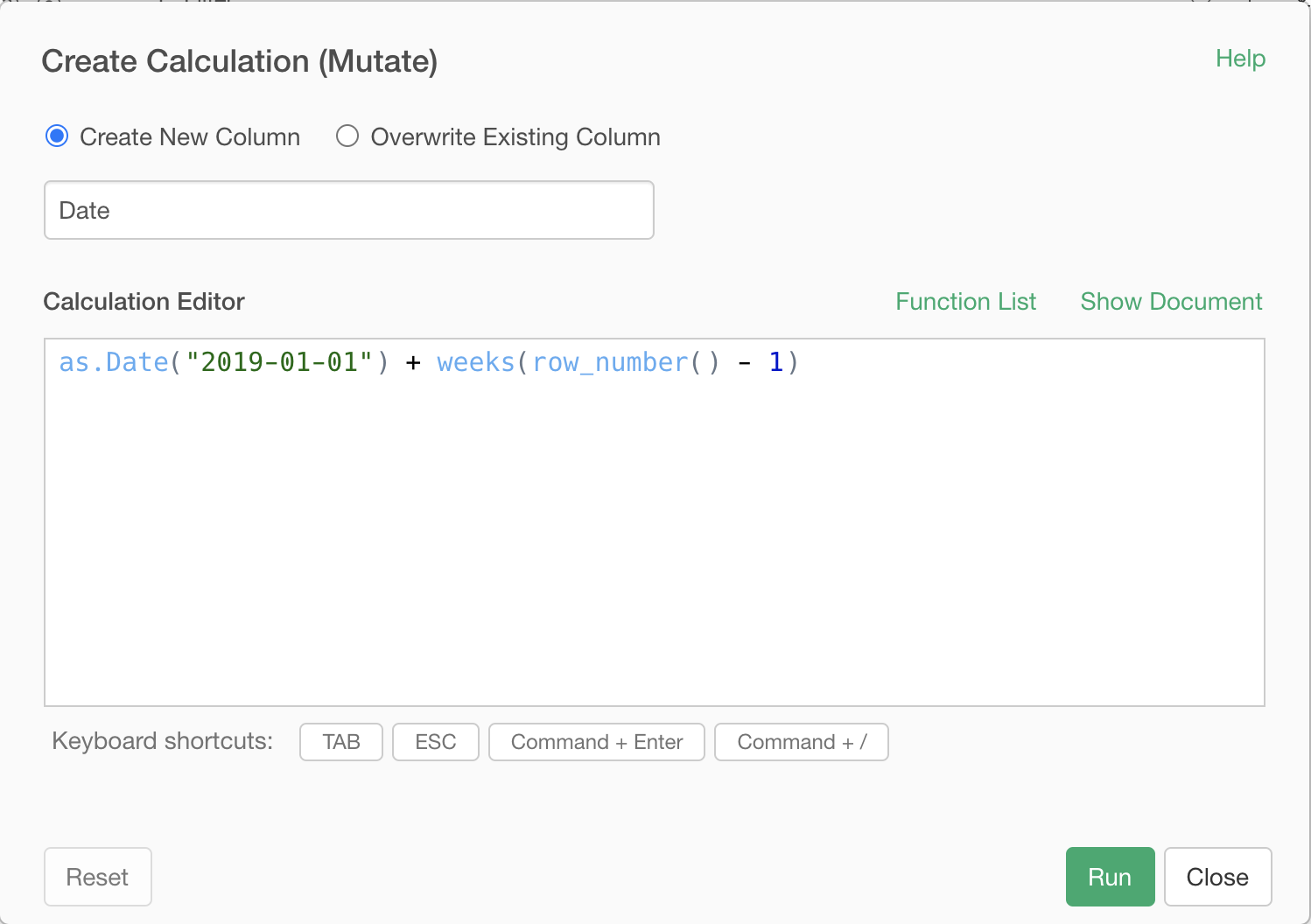

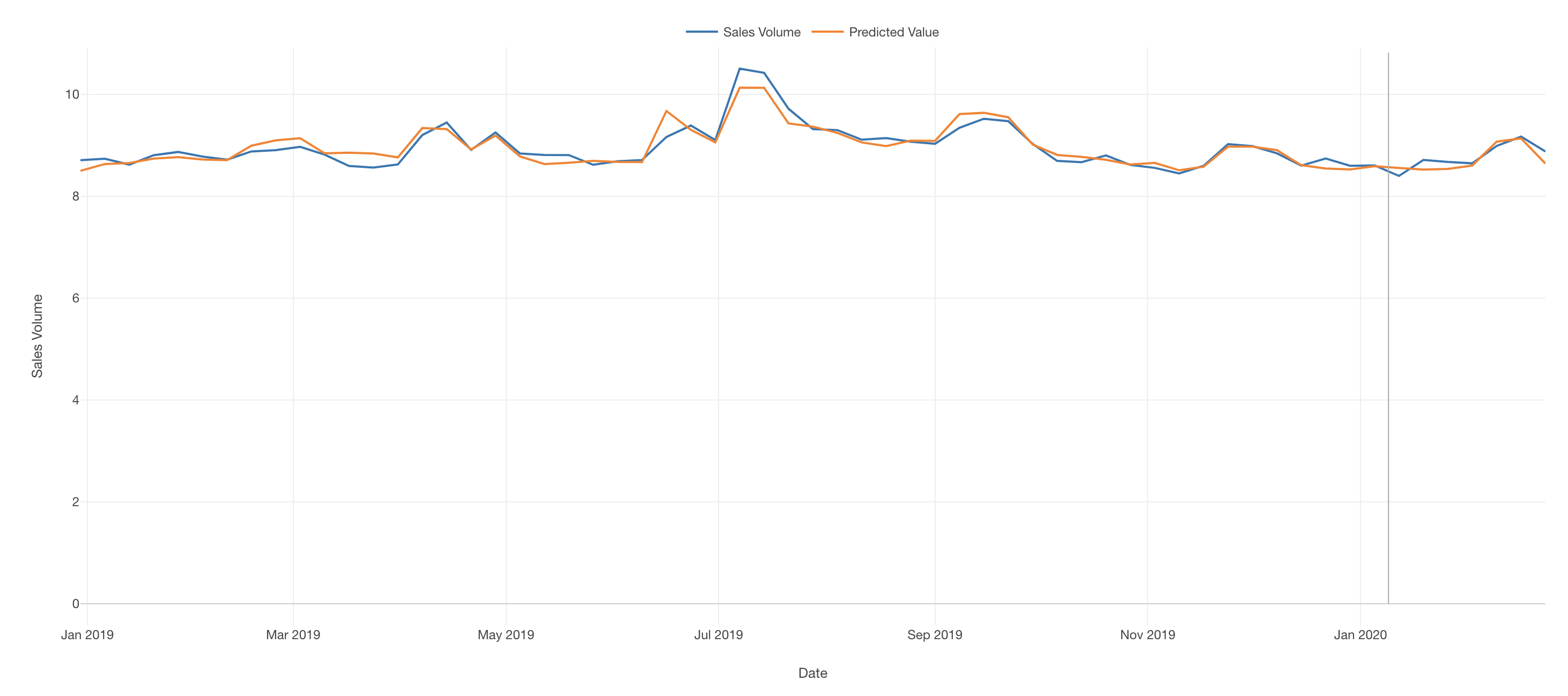
Let's create a line chart and set the columns for it like the following screenshot.

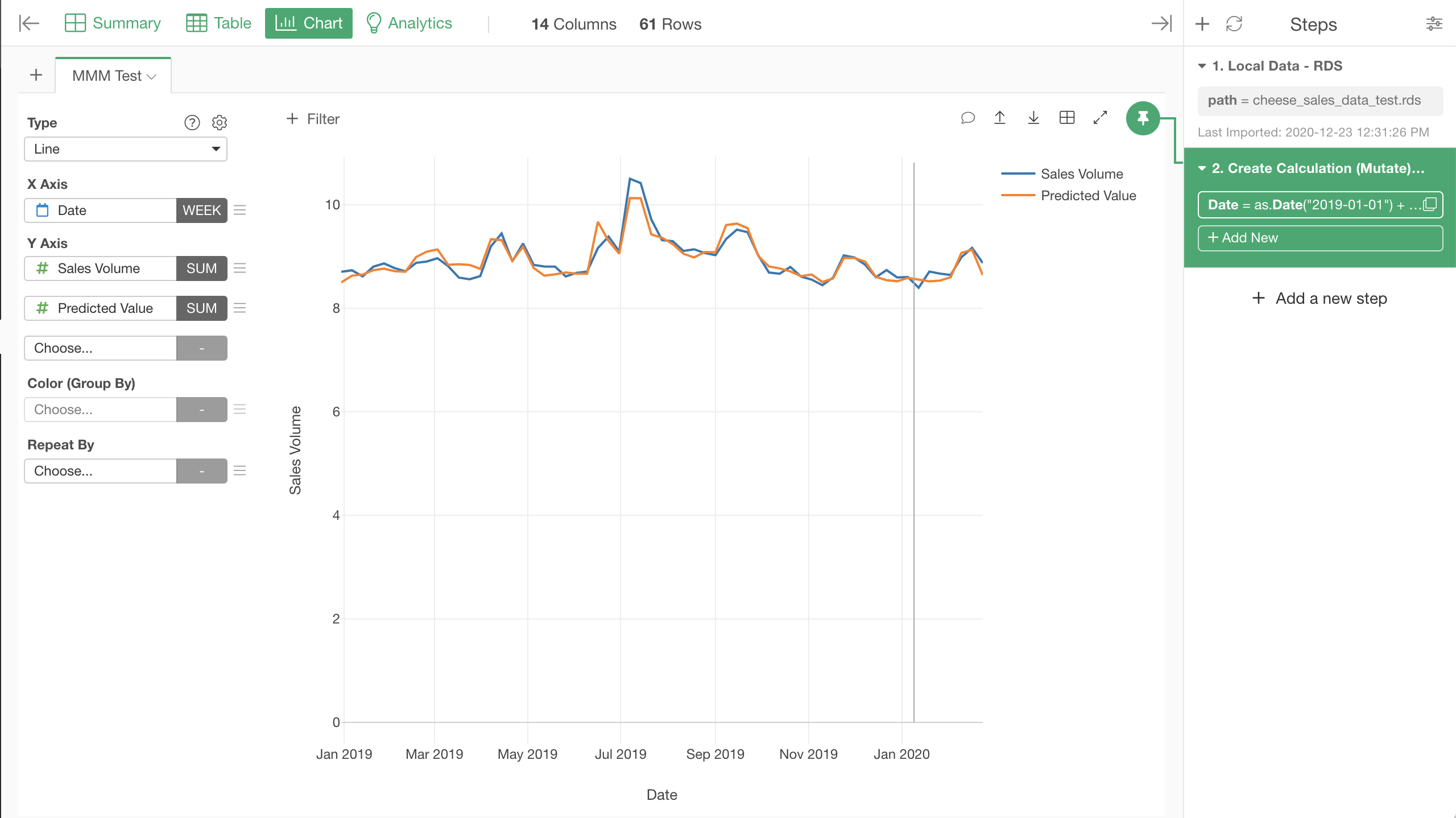
I also added a vertical reference line to distinguish between the period for the training data and the period for the test data. After the vertical line, the orange line was predicted by the model, without knowing the actual sales volume. It seems the sales volume is pretty well predicted.

Just for comparison, here is the same chart with the previous model which was without adstock.

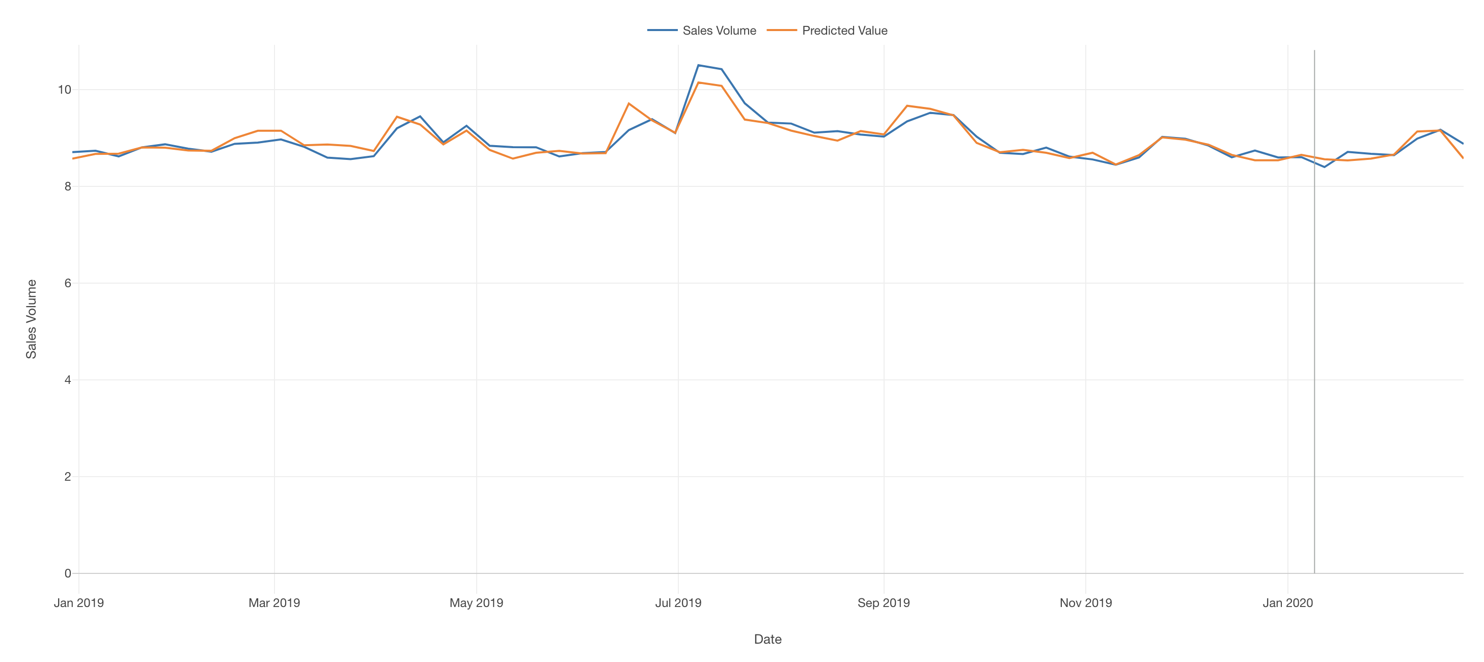
The difference is not very visible from the chart, but it had slightly lower test R squared of 71% compared with our latest model with test R squared of 77%. Here is the Summary table from the model without adstock, again for comparison.

Predict with the Model

Now, making use of the model we got, let's predict future sales volume given certain future plan on advertisement and pricing.

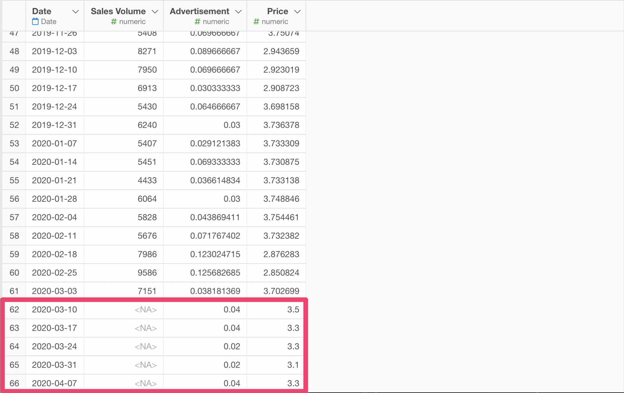
Let's say we planned the advertisement and pricing for the next 5 weeks as in this new data, which is the original data plus those 5 rows for the future planning. Since this is for the future, the Sales Volume values are NAs. We are to predict those values based on the planned advertisement and pricing with the model we previously built.

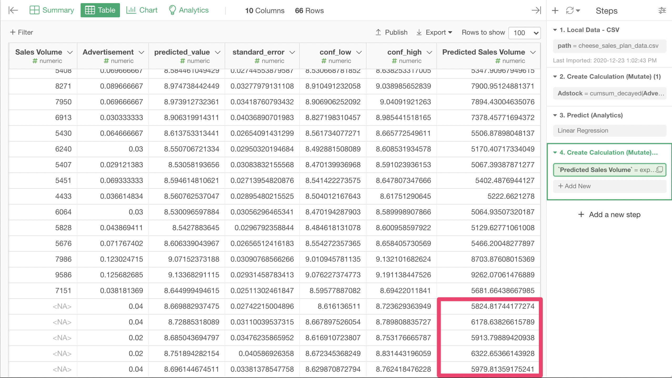
To make the model work, we had to calculate the adstock first. We can do so by copying and pasting the step we calculated the adstock when we built the model to this Data Frame.

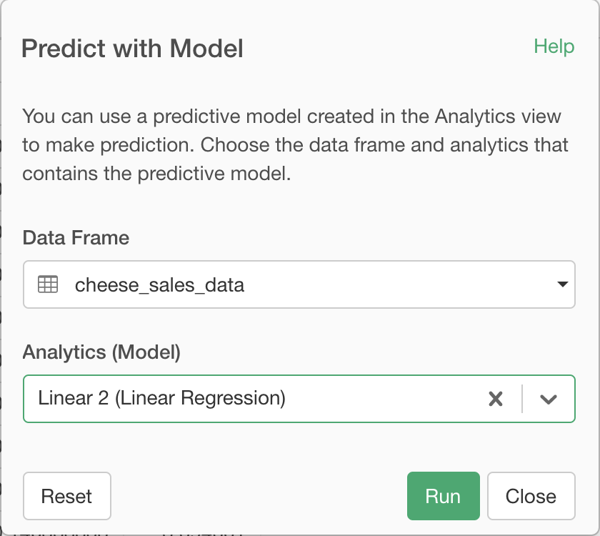
Let's make a prediction with the model. Before this step, I turned off the Test Mode of the model in the Analytics View, so that all the past data is used for the training of the model. Now, follow the menu like the screenshot to open Predict with Model (Analytics View) dialog.

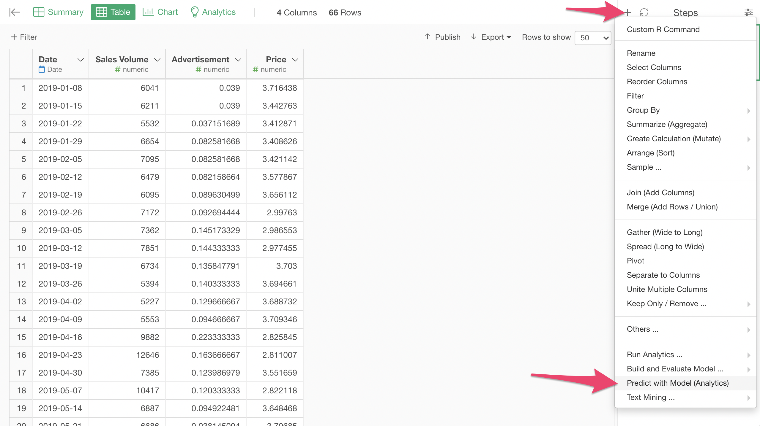
In the dialog, specify the model, by the Data Frame it was built upon and the Analytics View for it. Click the Run button to make the prediction.

We can see that the predicted_value colum has the predicted values for the last 5 rows.

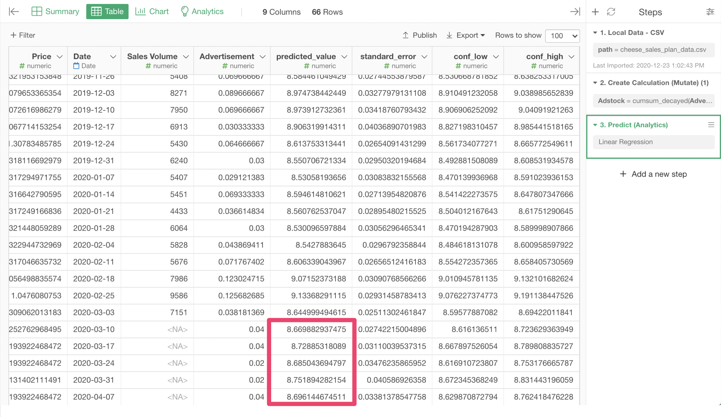
The predicted values of this model was log of sales volume. To calculate the prediction for the raw sales volume, we need to apply exponential function, which is the reverse of the log function, by the following expression.

exp(predicted_value)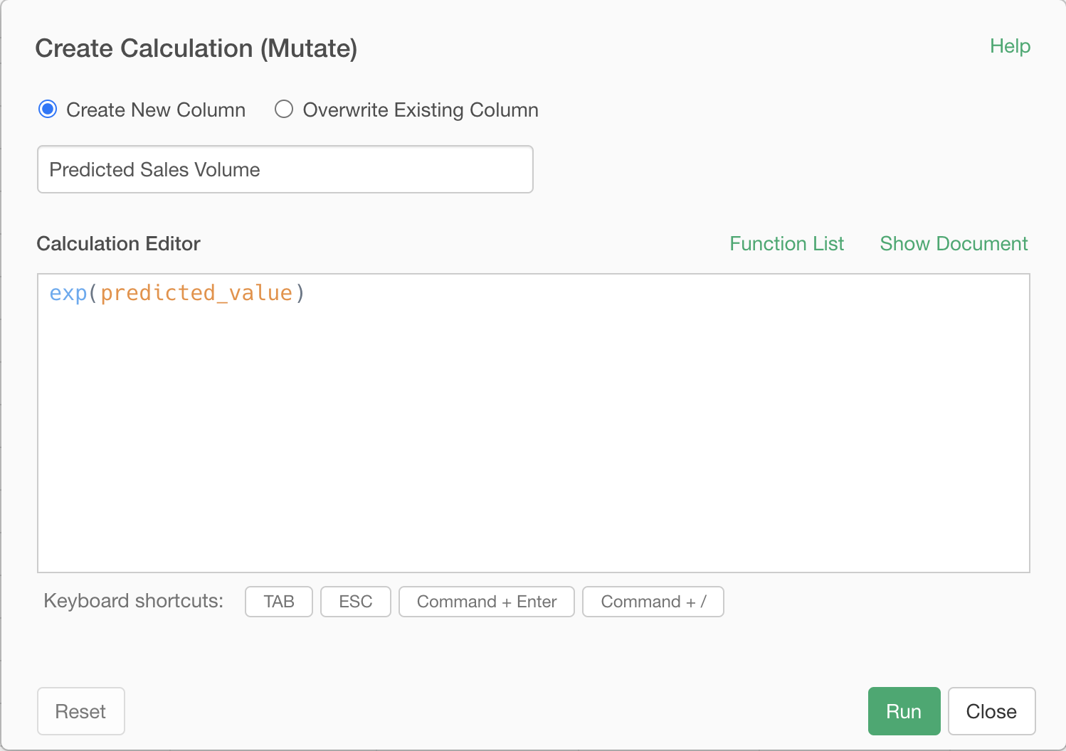

Now we have the prediction for the raw sales volume for the weeks we made the plan for!

Let's visualize this with line chart, by specifying the columns for it like the screenshot.

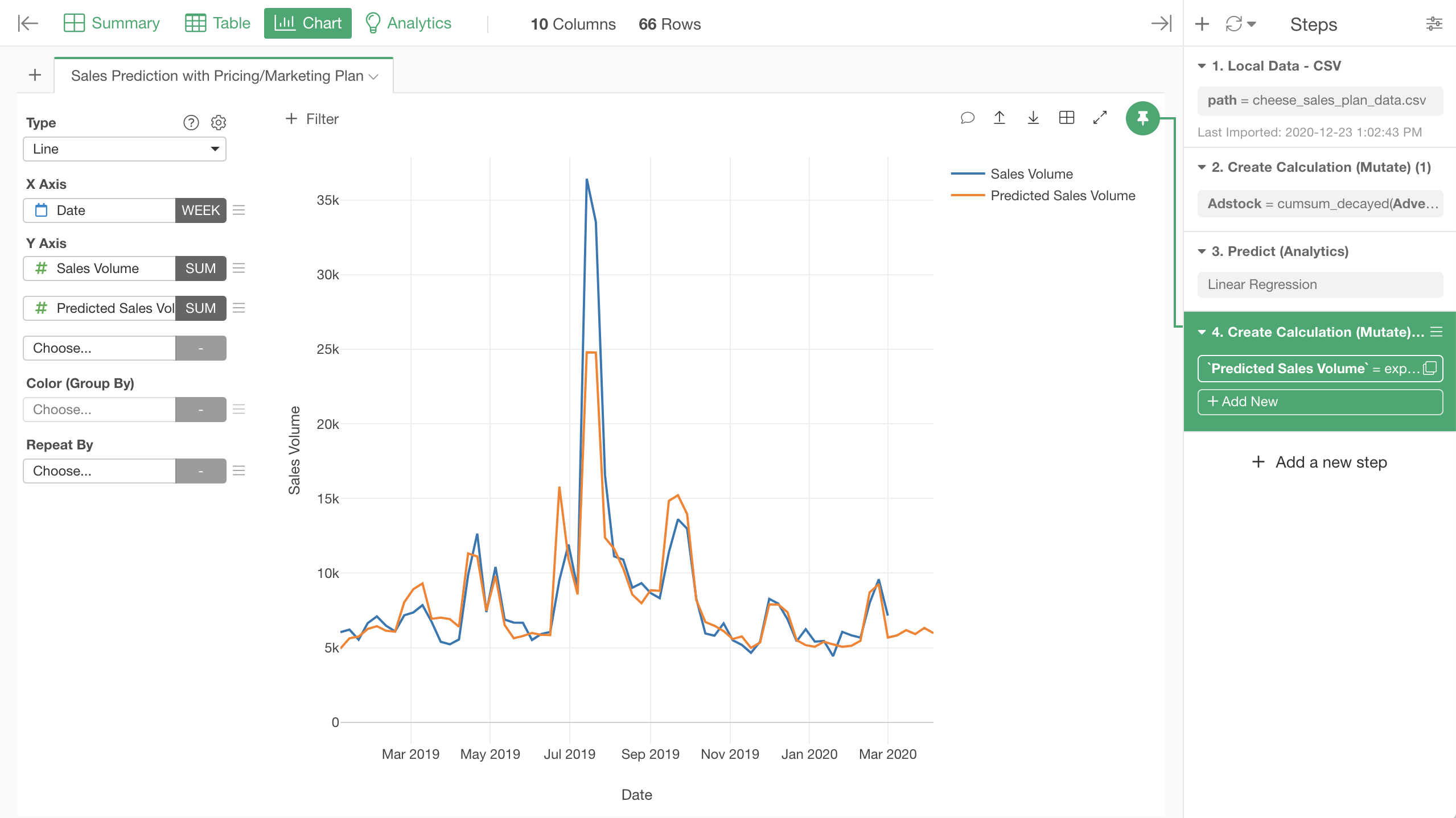
Here is a better view of the same line chart. The last 5 weeks, which only has the orange predicted values is the period that the model predicted.

Conclusion

In this article, I explained how to build Marketing Mix Model, making use of Linear Regression Analytics View of Exploratory with some data wrangling. Our model models the relationship between pricing and sales with the assumption of constant price elasticity. It models the relationship between advertisement and sales with adstock calculated based on decaying carry over effect of advertisement.

In the next post in this series, I will explain about building Marketing Mix Model with time series forecasting with Prophet algorithm with Exploratory. With that we should be able to handle the effect of trend and seasonality too. Stay tuned!